Confidence Intervals

Let’s first set out an example. Online courses seem to love the example of someone trying to measure the IQ of some population so I’ll try and mix it up a little. Let’s say we are trying to estimate the mean monthly rent for a property in London (in £). We could try to get the exact value by asking everyone in London but that seems a little cumbersome, so instead we will simply ask a sample of people.

Once we have our sample there are a number of ways we can calculate a confidence interval ( see here for some examples) but I want to focus on the interpretation, so we’ll be using a t-distribution. We can calculate the 95% confidence interval as follows:

# Set the true mean and standard deviation
mu <- 1200 # That's £1200 a month
sd <- 300   # With a standard deviation of 300
n <- 30    # We manage to sample 30 people in London
set.seed(23)
# We simulate collecting this sample
sample <- rnorm(n=n, mean=mu, sd=sd)
# We identify the sample mean (which will differ from the true mean)
sample_mean <- mean(sample)
sample_sd <- sd(sample)

# We can then calculate the confidence interval by subtracting and adding
# this error term to the sample mean respectively
error <- qt(1 - (0.05/2), df=n-1)*sample_sd/sqrt(n)
cat(
    paste0(
        "The sample mean is: ", round(sample_mean, 2),
        "\nThe 95% CI is: [", round(sample_mean - error ,2), ",",
        round(sample_mean + error, 2), "]"
    )
)
## The sample mean is: 1247.17
## The 95% CI is: [1153.12,1341.22]

So after asking 30 people we find that the mean rent is £1247.17, with a 95% CI of [1153.12, 1341.22]. It may be tempting to think that this means there is a 95% chance the true population mean is in that range, but this isn’t right. In fact we already know from the way we constructed our simulation that the true mean is £1200, and as such it is definitely in that range! This is true even when we don’t set the value for ourselves, in reality the “true” value is fixed and it is either definitely in our interval or definitely not.

So then what does the interval mean? Actually it is relatively simple, it tells us how often in the long run the true mean will actually fall inside the interval. If you continually do experiments such as the one above and report 95% confidence intervals, 95% of the time the true population parameter (in our case the true mean rent in London) will be in that confidence interval.

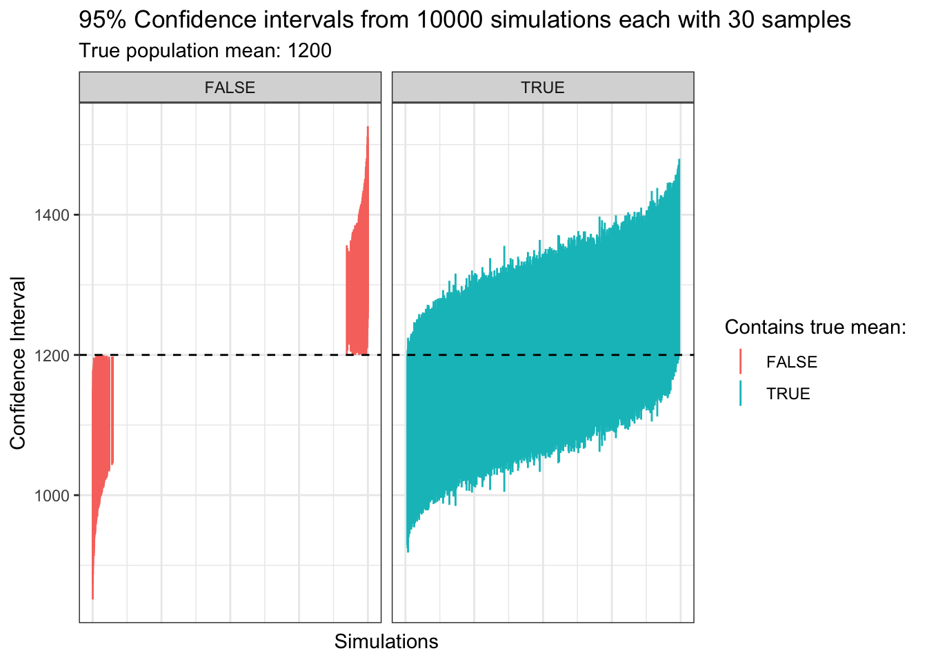
Let’s make that a little more visual. Suppose we did this simulation sample of 30 people over and over again on the same population, how would all the confidence intervals look then?

# Let's run the simulation of sampling of 30 people 10000 times
n_simulations <- 10000
# For each simulation we record the confidence interval
ci_lower <- numeric(n_simulations)
ci_upper <- numeric(n_simulations)
means <- numeric(n_simulations)
set.seed(23)
for(sim in seq(n_simulations)){
    # Run the simulation
    x <- rnorm(n=n, mean=mu, sd=sd)
    # Calculate the error term
    means[sim] <- mean(x)
    sample_sd <- sd(x)
    error <- qt(1 - (0.05/2), df=n-1)*sample_sd/sqrt(n)
    # Save the confidence intervals
    ci_lower[sim] <- means[sim] - error
    ci_upper[sim] <- means[sim] + error
}
# Group them together and order by the lower interval
simulations <- data.table(
    mean = means, ci_lower = ci_lower, ci_upper = ci_upper
)
simulations <- simulations[order(means)]
simulations$row_num <- 1:n_simulations

# Identify for each simulation if the CI contains the true mean
simulations[, contains_true_mean := ((ci_lower <= mu) & ( ci_upper >= mu))]

# Plot intervals
ggplot(simulations) +
    geom_linerange(
        aes(x=row_num, ymin=ci_lower, ymax=ci_upper, col=contains_true_mean)
    ) +
    geom_hline(yintercept=mu, linetype="dashed") +
    theme_bw() +
    labs(
        x="Simulations",
        y="Confidence Interval",
        col="Contains true mean:",
        title=paste0(
            "95% Confidence intervals from ", n_simulations,
            " simulations each with ", n, " samples"
        ),
        subtitle=paste0("True population mean: ", mu)
    ) +
    facet_grid(~contains_true_mean) +
    theme(axis.text.x=element_blank(), axis.ticks.x=element_blank())

After 10000 simulations we can see that many of our sample confidence intervals did contain the true population mean, and some did not. In fact the exact proportion was 94.99 %. This is where our 95% comes from. In the long run if we keep constructing 95% confidence intervals for different samples then they will contain the true population parameter (in our case the mean rent) 95% of the time!

The unfortunate thing is that normally in an experiment you will only do this sampling once. As such you will only build one confidence interval and you may end up building one that doesn’t contain the true mean, all that time sampling and you may be missing the true value. But you know from that sampling that different true values are possible, sure it doesn’t seem very likely given the data that the true value is actually true but it’s still possible, wouldn’t it be nice to see how likely any value is? This is more suited to the field of Bayesian statistics which we will see more of in the next section.

Credible Intervals

This is where it gets a little tough for me, but I will give my interpretation of the difference between this intervals.

Credible intervals come from the world of Bayesian statistics (contrary to the frequentist background of confidence intervals). Frequentist statistics, much like as we used in the example above, focuses on a single population parameter (e.g. the mean rent in London) and tries to capture this parameter accurately over a number of experiments. For each experiment we say we have some confidence our true parameter is in a given interval, and expect to be incorrect a certain percentage of experiments.

The Bayesian approach looks at the parameter as a random variable, namely that different values of this parameter all have different likelihoods of being true. Sure we may have observed in our sample that the mean rent in London is £1247 a month but we still think there is some likelihood about other values. A population mean of £1000 is still possible, and even £2000 with some lesser probability.

What is unusual is that in the case we use an uninformative prior for the Bayesian approach, we actually get the same interval as the confidence interval. So what is a prior? This is in fact just a probability distrubition that says how likely each parameter is before we’ve seen the data. An uninformative prior says that we have no idea which values are more likely than another before we sample. But practically this isn’t true, is a mean monthly rent of £1200 really as likely as £200? Intuitively we think that £1200 is more likely either from anecdotal stories or some past data we might have seen.

In Bayesian statistics we take this prior belief (a distribution) and update our belief using observed data (our samples). The result is what is known as a posterior distribution. It tells us the probability of any parameter value being true given the data we’ve observed. Then what is a credible interval? This is a range of parameter values that cover 95% of the posterior probability mass.

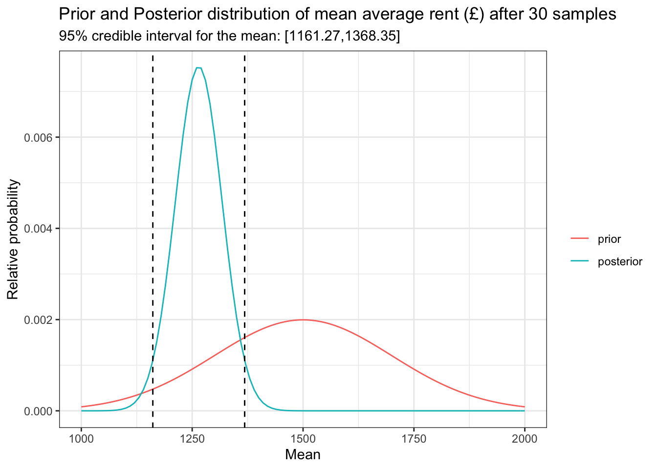
This may be a little hard to follow so let’s extend our example above. We will simulate collecting the rent data for 30 households like before, but we will also incorporate a prior. Let’s say we assume £1500 is most likely but we don’t have too much certainty in this (we quantify this level of certainty through the prior’s variance). Let’s see below how this looks when we create a posterior distribution:

# Let's set up a range of parameter values. We say we want to know likelihood
# values for parameters (mean monthly rent) between £1000 and £2000 in steps of
# £10
param_vals <- seq(1000, 2000, 10)
# We firstly set up our prior
prior_mu <- 1500 # We assume a mean of £1500 per month
prior_sd <- 200  # But we don't know very strongly that that is the case
# NOTE: this standard deviation shows our certainty around the value of the
# mean, it does not express our belief about how the actual population mean
# deviates. For example if we set this value to 0 that means we believe that
# 1500 is the true value, and there is zero probability of any other value
# being true.

# We get the prior probability of each parameter value
prior_probabilities <- dnorm(param_vals, mean=prior_mu, sd=prior_sd)

# Let's use our same 30 person sample as before, the variable was called
# "sample"

# Now using the prior and our data we can construct a posterior distribution
# using our normal conjugate prior and the following formulae:
# https://en.wikipedia.org/wiki/Conjugate_prior#Table_of_conjugate_distributions
posterior_mu <- ((prior_mu/(prior_sd^2)) + (sum(sample)/(sd^2)))/
                ((1/prior_sd^2) + (n/(sd^2)))
posterior_sigma <- 1/((1/(prior_sd^2)) + (n/(sd^2)))
posterior_probabilities <- dnorm(
    param_vals, mean=posterior_mu, sd=sqrt(posterior_sigma)
)

# Now combine all 3 together
bayesian_update <- data.table(
    vals = param_vals,
    prior = prior_probabilities,
    posterior = posterior_probabilities
)

# Calculate the 95% credible interval
ci_lower <- qnorm(0.05/2, mean=posterior_mu, sd=sqrt(posterior_sigma))
ci_upper <- qnorm(1-(0.05/2), mean=posterior_mu, sd=sqrt(posterior_sigma))

ggplot(melt(bayesian_update, id="vals"), aes(x=vals, y=value, col=variable)) +
    geom_line() +
    geom_vline(xintercept = ci_lower, linetype="dashed") +
    geom_vline(xintercept = ci_upper, linetype="dashed") +
    theme_bw() +
    labs(
        x="Mean",
        y="Relative probability",
        col="",
        title=paste0(
            "Prior and Posterior distribution of mean average rent (£) after ",
            n, " samples"
        ),
        subtitle=paste0(
            "95% credible interval for the mean: [",
            round(ci_lower, 2), ",", round(ci_upper, 2), "]"
        )
    )

Well that’s interesting. This method tells us that our credible interval is [1161.27, 1368.35]. We found that by chopping the posterior curve at points that leave 95% of the area under the curve (probability mass). Technically this isn’t a unique area but given that the normal distrubution is symmetric about the mean then we can just chop an equal distance either side of the mean. Compare that to the confidence interval we calculated earlier which was [1137.96, 1356.38].

In this method we said that our prior knowledge tells us that £1500 is a possible mean, but we aren’t really that certain and we think that values that are a few hundred £ either side are also very possible. Then we observed our 30 samples like before and used that to update our belief. This created our “posterior” which is a lot more narrow. This says we are a bit more certain which range of values are actually realistic. Notice that our credible interval is actually a little higher than the confidence interval. That is because we don’t totally discard our prior belief that £1500 is a sensible mean, we simply update our belief depending on how much new data we saw.

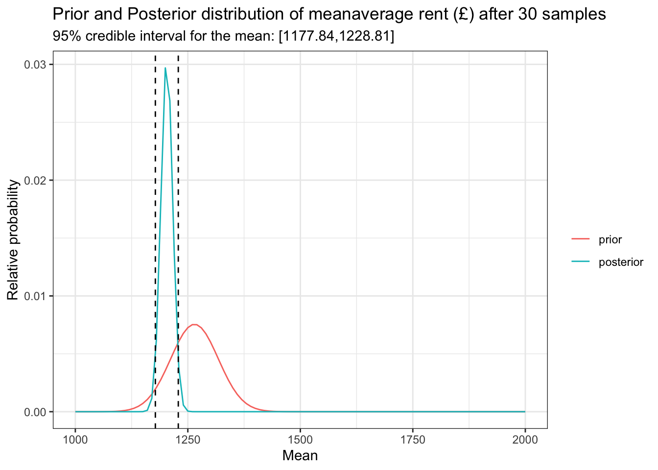
Just for interest we can pretend that we keep sampling until we get lots and lots of data. The beauty of Bayesian updating is that we use this posterior above as a prior (it’s our latest belief about what is true) and update it with new data to create a new posterior!

# Let's sample 500 more people
n2 <- 500
new_sample <- rnorm(n=n2, mean=mu, sd=sd)

# We turn our posterior into a prior
prior_mu <- posterior_mu
prior_sd <- sqrt(posterior_sigma)
prior_probabilities <- dnorm(param_vals, mean=prior_mu, sd=prior_sd)

# Now let's do the update again
posterior_mu <- ((prior_mu/(prior_sd^2)) + (sum(new_sample)/(sd^2)))/
                ((1/prior_sd^2) + (n2/(sd^2)))
posterior_sigma <- 1/((1/(prior_sd^2)) + (n2/(sd^2)))
posterior_probabilities <- dnorm(
    param_vals, mean=posterior_mu, sd=sqrt(posterior_sigma)
)

# Now combine all 3 together
bayesian_update2 <- data.table(
    vals = param_vals,
    prior = prior_probabilities,
    posterior = posterior_probabilities
)

# Calculate the 95% credible interval
ci_lower <- qnorm(0.05/2, mean=posterior_mu, sd=sqrt(posterior_sigma))
ci_upper <- qnorm(1-(0.05/2), mean=posterior_mu, sd=sqrt(posterior_sigma))

ggplot(
    melt(bayesian_update2, id="vals"), aes(x=vals, y=value, col=variable)
) +
    geom_line() +
    geom_vline(xintercept = ci_lower, linetype="dashed") +
    geom_vline(xintercept = ci_upper, linetype="dashed") +
    theme_bw() +
    labs(
        x="Mean",
        y="Relative probability",
        col="",
        title=paste0(
            "Prior and Posterior distribution of mean",
            "average rent (£) after ",
            n, " samples"
        ),
        subtitle=paste0(
            "95% credible interval for the mean: [",
            round(ci_lower, 2), ",", round(ci_upper, 2), "]"
        )
    )

Look at that. Now we are saying that the most likely range of values for which our true mean is lies between £[1177.84, 1228.81] which is quite tight around our true value of 1200.

Conclusion

Interpreting statistics is a minefield, both in complexity and danger. When you reflect on the fact that statistics such as these are important for things such as medical research it’s clear that the consequences of misinterpreting values can have dire consequences. When we later come to visit P-values we’ll see that not being careful can lead us to make mistakes well over 5% of the time even using an alpha level of 95%.

In the world of intervals it is equally difficult to know which path to follow. If you base business decisions on frequentist statistics (e.g. P-values and confidence intervals) then you expect to make wrong conclusions for a fixed amount of experiments, but that’s fine because if you do everything right you can control for it. If you take a Bayesian approach you can incorporate prior beliefs such as previous test or just sensibility checks, you can also express your estimation of some value as a range of probabilities - sure you ran your test for 6 months and see a clear effect emerging but there is some probability, no mattter how small, that the real effect size is 0. Nevertheless you still have to set some decision criteria otherwise you will never end a test and accept a new feature, and because of that sometimes you will be wrong still!

I hope I did these intervals some justice, and I welcome some robust review of what I wrote above. I am basing this on recently-enhanced knowledge and reading a mixture of articles to confirm my understanding, and the fact is I am either completely right about what I wrote or have made some mistake. In my mind I have established some credibility about what I wrote and my arbitrary decision criteria has lead me to post this.